A Lutin Tutorial
Table of Contents
- 1 Forewords
- 2 Execute Lutin programs
- 3 The Lutin Language
- 3.1 Back to programs of Section 1
- 3.2 Non deterministic programs
- 3.3 Non deterministic programs (cont)
- 3.4 Non deterministic programs (cont)
- 3.5 Non deterministic programs (cont)
- 3.6 Controlled non-determinism: the choice operator
- 3.7 Controlled non-determinism: the choice operator
- 3.8 Combinators
- 3.9 A parametric combinator
- 3.10 Combinators (cont)
- 3.11 Local variables
- 3.12 Local variables again
- 3.13 Damped oscillation
- 3.14 Distribute a constraint into a scope:
assert - 3.15 External code
- 3.16 Exceptions
- 3.17 Exceptions (cont)
- 3.18 Exceptions (cont)
- 3.19 Combinators (again)
- 3.20 Parallelism:
&>
- 4 The
runoperator - 5 Advanced examples
1 Forewords
1.1 Motivations: testing reactive programs
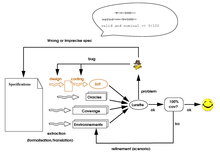
Lutin aims at facilitating the writing of SUT environments, seen as non-deterministic reactive machines.
1.2 Lutin in one slide
- Lustre-like: Dataflow, parallelism, modular, logic time,
pre. - But not exactly Lustre though
- Plus
- Control structure operators (regular expressions)
- Stochastic (controlled and pseudo-Aleatory)
- Minus
- No implicit top-level loop
- No topological sort of equations
- Plus
1.3 In order to run this tutorial
You first need to install opam. For instance, on debian-like boxes do
sudo apt-get install opam
opam init ; opam switch 4.04.0 ; eval `opam config env`
and then do:
sudo apt-get install gnuplot tcl
opam repo add verimag-sync-repo "http://www-verimag.imag.fr/DIST-TOOLS/SYNCHRONE/opam-repository"
opam update
opam install lutin
and also the Lustre V4 distribution (for luciole and sim2chro) http://www-verimag.imag.fr/DIST-TOOLS/SYNCHRONE/lustre-v4/distrib/index.html
Basically, to get all the tools necessary to run this tutorial accessible
from ypour path, you should have something like that in your .bashrc :
# for lutin, gnuplot-rif, luciole-rif
. ~/.opam/opam-init/init.sh > /dev/null 2> /dev/null || true
# for simec (luciole), sim2chrogtk
export LUSTRE_INSTALL=~/lustre-v4-xxx
source $LUSTRE_INSTALL/setenv.sh
1.4 In order to run the demo from the pdf slides
You can edit (on linux boxes) your ~/.xpdfrc resource
file modify the urlCommand rule:
urlCommand "browserhook.sh '%s'"
- Download the bash script browserhook.sh (link to the script)
- Make it executable and available from your path
- Then the green link should launch the corresponding shell command,
2 Execute Lutin programs
2.1 Stimulate Lutin programs
Before learning the language, let's have a look at a couple of tools that will allow us to play with our Lutin programs.
The Lutin program command-line interpreter is a stand-alone
executable named lutin. This program ougth to be
accessible from your path if you have followed the instr
- A program that increments its input
Let's consider the following Lutin program named incr.lut.
node incr(x:int) returns (y:int) =
     loop [10] y = x+1
<prompt> lutin incr.lut
# This is lutin Version 1.54 (9e783b6)
# The random engine was initialized with the seed 817281206
#inputs "x":int
#outputs "y":int
#step 1
This is a reactive program that returns its input, incremented by 1, forever. We'll explain why later. For the moment, let's simply execute it using
lutinfrom a shell:At this stage,
lutinwaits for an integer input to continue. If we feed it with a1(type1<enter>), it returns 2. If we enter 41, it returns 42. To quit this infinite loop gently, just enter the characterq.<promt> lutin incr.lut $ 1 1 #outs 2 #step 2 $ 41 41 #outs 42 #step 3 $ q q# bye! #end.
- A program with no input
node one() returns (y:int) =
   loop y = 1
<prompt> lutin -l 5 one.lut
# This is lutin Version 1.54 (9e783b6)
# The random engine was initialized with the seed 931220738
#inputs
#outputs "y":int
#step 1
#outs 1
#step 2
#outs 1
#step 3
#outs 1
#step 4
#outs 1
#step 5
#outs 1
A Lutin program might have no input at all. In such a case, it might be to helpful to know that the
--max-steps(-lfor short) allows one to set a maximum number of simulation steps to perform.Question : Try to launch
lutin one.lut -l 5on one.lut
- Be quiet
<prompt> lutin -l 5 -quiet one.lut
1
1
1
1
1
The previous simulation basically produces a (wordy) sequence of five "1". To obtain quieter sequence, one can use the
-quietoption (-qfor short):
2.2 Stimulate Lutin programs graphically with luciole
node incr(x:int) returns (y:int) =
     loop [10] y = x+1
<prompt> luciole-rif lutin incr.lut
It is also possible to feed Lutin programs with luciole, a tcl/tk
based GUI that was originally crafted for Lustre programs. You will
need to have tcl/tk installed to be able to use it.
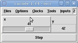
The use of Luciole is straightforward. Some useful features that you should try to play with are:
- The "Compose" mode (accessible via the "Clocks" menu)
- The "Real Time Clock" mode (accessible via the "Clocks" menu)
- The Sim2chro display (accessible via the "Tools" menu)
2.3 Store and Display the produced data: sim2chro and gnuplot-rif
- Generate a RIF file
It is possible to store the lutin RIF output into a file using the
-ooption.<prompt> lutin -l 10 -o ten.rif N.lut ; ls -lh ten.rif
node N() returns (y:int) =
   y = 0 fby loop y = pre y+1
- Visualize a RIF file
<prompt> cat ten.rif
The
#outs,#in, etc., produced bylutinare RIF directives. RIF stands for "Reactive Input Format"
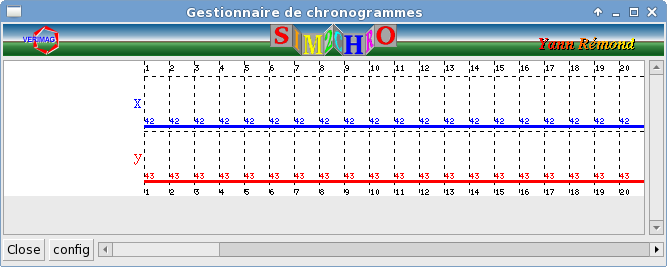
- Visualize a RIF file (bis)
<prompt> cat ten.rif | sim2chrogtk -ecran > /dev/null
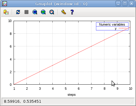
In order to graphically display the content of this .rif file, one can use two tools that are part of the
lutindistribution:sim2chro(orsim2chrogtk), andgnuplot-rif(requires gnuplot).
- Visualize a RIF file (ter)
<prompt> gnuplot-rif ten.rif
2.4 Automatic stimulation of Lutin programs
node incr(x:int) returns (y:int) =
     loop y = x+2
node decr(y:int) returns (x:int) =
     x = 42 fby loop x = y-1
<prompt> lurette -sut "lutin decr.lut -n incr" -env "lutin decr.lut -n decr" -o res.rif
<prompt> sim2chrogtk -ecran -in res.rif > /dev/null

- I've bought 2 electronic chess games
- connected one to another
- And now I'm at peace
3 The Lutin Language
The aim of this tutorial is to be complementary to the Reference Manual. The idea here is to present the language via examples. If you want precise definitions of the various language statements syntax and semantics, please refer to the Reference Manual.
3.1 Back to programs of Section 1
- Let's come back to the Lutin programs mentioned so far.
node incr(x:int) returns (y:int) =
     loop [10] y = x+1
- We said said that the first one, incr.lut increments its input by one. Let's explain why.
- Those programs illustrate the 2 kinds of expressions we have in Lutin.
- constraint expressions (
y = x+1) that asserts facts outputs variables. - trace expression (
loop<te>) that allows one to combine constraint expressions.
- constraint expressions (
The behavior of a satisfiable constraint expression is to produce as outputs one of its possible solutions during one logical instant (i.e., during one step). The behavior of the trace expression
loop teis to behave asteas long asteis satisfiable.Hence, the Lutin program incr.lut could be read like that:
I am a reactive program that takes an integer variable in input, and that returns an integer output. As long as possible, I will use the constraint
y = x+1to produce my output.Since this constraint always has a solution, that program will loop forever. Since this constraint has exactly one solution, this program is deterministic.
Now let's have a look at the second program we've seen.
node N() returns (y:int) =
   y = 0 fby loop y = pre y+1
The program N.lut illustrates the use of two central Lutin keywords:
fbyandpre.fbyis the trace sequence operator.b1 fby b2means: behaves asb1, and when no more behavior is possible, behaves asb2. The constrainty=0is always satisfiable; its behavior is to bind the outputyto 0 for one step.y=0 fby loop y = pre y+1will therefore behave asy=0for the first step, and asloop y = pre y+1for the remaining steps.preis the delay operator (as in Lustre).pre yis an expression that is bound to the value ofyat the previous instant.y = pre y+1will therefore increment the value ofyat each instant. Again this program is deterministic and runs infinitely.Of course, this means that
yshould be defined at the previous instant. This is the reason why we've distinguished the first step from the others. However, it is possible to set variables previous values at declarations time. The program N2.lut below behaves exactly as N.lut:node N2() returns (y:int = -1) = loop y = pre y+1
Question: Write a Lutin program with no input that generates one output
ywith the following sequence of values : 1 3 5 7 9 …Question: Write a Lutin program with no input that generates one output
ywith the following sequence of values : 1 2 4 8 16 32 … - Those programs illustrate the 2 kinds of expressions we have in Lutin.
3.2 Non deterministic programs
- A First non-deterministic program
node trivial() returns(x:int; f:real ; b:bool) =
  loop true
<prompt> lutin -l 10 -q trivial.lut
<prompt>  lutin -l 10 -q trivial.lut
129787787 89770690.47 f
-202124065 60018934.21 t
-74063075 -224861409.44 t
-120351222 37052102.10 t
-84618074 238667445.54 t
186689955 -188684349.70 t
211369478 -253941536.69 t
-135268511 52434720.53 t
113139954 241863809.02 t
-114970522 -70907151.75 t
The programs we've seen so far were deterministic because all the constraint expression were affectations (i.e., equalities between an input and an output variables). As a matter of fact, writing non-deterministic is even simpler: you just need to write no constraint at all! Indeed, observe how this trivial.lut program behaves:
- It is possible to set the variable range at declaration time,
as done in trivial2.lut:node trivial() returns(x:int [-100;100]; f:real [-100.0;100.0];b:bool)= loop true
<prompt> lutin -l 10 -q trivial2.lut
71 42.08 f
-61 27.28 f
-49 -64.96 f
44 63.08 t
-15 73.06 f
0 -74.39 f
87 -1.58 f
-20 89.62 f
3 -84.20 t
89 28.64 f
3.3 Non deterministic programs (cont)
As you've just seen, a Lutin program is by default chaotic. To make it less chaotic, one has to add constraints which narrow the set of possible behaviors. When only one behavior is possible, the program is said to be deterministic. When no behavior is possible, the program stops.
Now consider the range.lut program:
node range() returns (y:int) = loop 0 <= y and y <= 42
<prompt> lutin range.lut -l 10 -q
The constraint expression 0 <= y and y <= 42 has several
solutions. One of those solutions will be drawn and used to produce
the output of the current step.
<prompt> lutin range.lut -l 10 -q
24
38
12
30
5
5
40
8
26
39
Lutin constraints can only be linear, which means that the set of solutions is a union of convex polyhedra. Several heuristics are defined to perform the solution draw, that are controlled by the following options:
--step-inside(-si): draw inside the polyhedra (the default)--step-vertices(-sv) draw among the polyhedra vertices--step-edges(-se): promote edges
<prompt> lutin range.lut -l 10 -q --step-vertices
42
0
42
42
0
42
42
0
0
42
Question: write a simpler program than range.lut that behaves the same.
3.4 Non deterministic programs (cont)
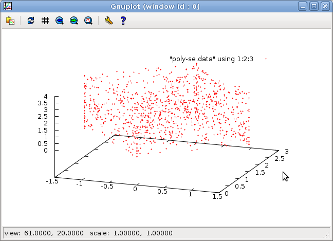
- A 3D non-deterministic example
Of course constraints can be more complex as in polyhedron.lut:
node polyhedron() returns(a,b,c:real) =
   loop (0.0 < c and c  < 4.0 and
         a + 1.0 * b > 0.0 and
         a + 1.0 * b - 3.0 < 0.0 and
         a - 1.0 * b < 0.0 and
         a - 1.0 * b + 3.0 > 0.0)
<prompt> lutin polyhedron.lut -l 1000 -q > poly.data;\\
echo 'set point 0.2; splot "poly.data" using 1:2:3;pause mouse close'| gnuplot
However, constraint expressions should be linear. For example, x * x >0 is rejected by the current solver. But of course, x * y > 0
is ok if x (or y) is an input.
gnuplot-rif is not designed to display 3d data; however, one can
generate and visualize data generated by this program using the 3D
plotting facilities of gnuplot like that:
- One can observe the effect of –step-edges
and –step-vertices ) options on the repartition of generated points
<prompt> lutin polyhedron.lut -l 1000 -quiet -se > poly-se.data
<prompt> lutin polyhedron.lut -l 1000 -quiet -sv > poly-sv.data
<prompt> echo 'set pointsize 0.2; splot "poly-se.data" using 1:2:3;pause mouse close'| gnuplot
<prompt> echo 'set pointsize 0.8; splot "poly-sv.data" using 1:2:3;pause mouse close'| gnuplot
hint: use the mouse inside the gnuplot window to change the perspective.
3.5 Non deterministic programs (cont)
Constraint may also depend on inputs.
Try to play the range-bis.lut program:
node range_bis(i:int) returns (y:int) =
   loop 0 <= y and y <= i
<prompt> luciole-rif lutin range-bis.lut
The major difference with range.lut is that the constraint
expression 0 <= y and y <= i is not always satisfiable. If one
enters a negative value, that program will stop.
Question: modify the range-bis.lut program (with the concept introduced so far) so that when a negative input is provided, it returns -1.
3.6 Controlled non-determinism: the choice operator
node choice() returns(x:int) =
   loop {
      | x = 42
      | x = 1
}
<prompt> lutin -l 10 -q choice.lut
42
42
42
1
42
42
42
42
1
1
In the previous programs, it is not possible to control the
non-determinism. It is possible to change the drawing heuristics,
but that's all. In order to control the non-determinism, one as
to use the choice operator (|).
When executing the choice.lut, the Lutin interpreter performs a
fair choice among the 2 satisfiable constraints (x = 42 and x = 1).
It is possible to favor one branch over the other using
weight directives (:3):
node choice() returns(x:int) =
   loop {
      |3: x = 42
      |1: x = 1
}
In choice2.lut, x=42 is chosen with a probability of 3/4.
<prompt> lutin -l 10000 -q choice2.lut | grep 42 | wc -l
7429
nb: "|" is a shortcut for "|1:".
nb 2: having 3 choices with a weight of 1, that does not necessarily means that each branch is chosen with a probability of 1/3. Indeed, the choice in done among satisfiable constraints. For instance in choice3.lut below, not all the branches of the alternative can be satisfiable.
3.7 Controlled non-determinism: the choice operator
node choice(b:bool) returns(x:int) =
   x=0 fby
   x=-15 fby
   loop {
      |1: x = 1 and b
      |9: x = 2 and b
      |   x = 3 and not b
}
<prompt> luciole-rif lutin choice3.lut
3.8 Combinators
A combinator is a well-typed macro that eases code reuse.
One can define a combinator with the let/in statement, or just
let for top-level combinators.
- A simple combinator
let n = 3

node foo() returns (i:int) =
  loop [3] 0<= i and i < n fby
  let s=10 in
  loop [3] s<= i and i < s+n
<prompt> lutin -quiet letdef.lut
3.9 A parametric combinator
The combinator.lut program illustrates the use of parametric combinators:
let within(x, min, max: int): bool =
  (min <= x) and (x <= max)

node random_walk() returns (y:int) =
  within(y,0,100) fby loop within(y,pre y-1,pre y+1)
<prompt> lutin -l 100 combinator.lut -o walk.rif ; gnuplot-rif walk.rif
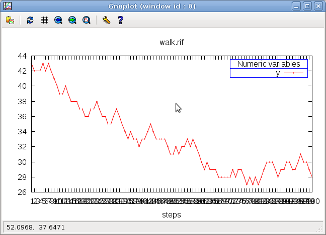
Question: Write such a randow walk for a real variable
3.10 Combinators (cont)
- A combinator that needs memory (
ref)
If one wants to access to the previous value of a variable inside a combinator, one has to declare in the combinator profile that this variable is a reference using the
refkeyword, as illustrated in the up-and-down.lut program:let within(x, min, max: real) :bool = (min <= x) and (x <= max) let up (delta:real;x:real ref):bool = within(x,pre x,pre x+delta) let down(delta:real;x:real ref):bool = within(x,pre x-delta,pre x) node up_and_down(min,max,d:real) returns (x:real) = within(x, min, max) fby loop { | loop { up (d, x) and pre x < max } | loop { down(d, x) and pre x > min } }
<prompt> luciole-rif lutin up-and-down.lut
<prompt> gnuplot-rif luciole.rif
The combinator
up(repsdown) constraints the variablexto be between its previous value and its previous value plus (resp minus) a positivedelta. The nodeup-and-down, after an initialization step wherexis drawn betweenminandmax, chooses (fairly) to go up, or to go down. It it chooses to go up, it does so as long asxis smaller thanmax; then it goes down, untilmin, and so on.Question: what happens if you guard the
upcombinator byx<maxinstead ofpre x < max?
3.11 Local variables
Sometimes, it is useful to use auxiliary variables that are not
output variables. Such variables can be declared using the
exist/in construct. Its use is illustrated in the
true-since-n-instants.lut program:
let n = 3
node ok_since_n_instants(b:bool) returns (res:bool) =
  exist cpt: int = n in
     loop {
       cpt = (if b then (pre cpt-1) else n) and
       res = (b and (cpt <= 0))
     }
<prompt> luciole-rif lutin true-since-n-instants.lut
It is possible to set its previous value at declaration time as for
interface variables. Here, the previous value of local variable cpt
is set to the constant n, which is bound to 3. This local variable is
used to count the number of consecutive instants where the input b
is true. cpt is reset to n each time b is false, and
decremented otherwise. The node returns true when cpt is smaller or
equal than 0.
3.12 Local variables again
The previous example was deterministic (it was actually a Lustre
program with an explicit loop), the local variable was a simple
(de)counter.
Local variables can also plain random variables, as illustrated the local.lut program:
node local() returns(x:real = 0.0) =
  exist target : real in
  loop {
    0.0 < target and target < 42.0 and x = pre x
    fby
    loop [20] { x = (pre x + target) / 2.0 and
                target = pre target }
  }
At first step, the local variable target is chosen randomly
between 0.0 and 42.0, and x keeps its previous value (0); then,
during 20 steps, the output x comes closer and closer to target (x = (pre x + target) / 2.0), while target keeps its previous value.
After 20 steps (loop [20])), another value for target is chosen,
and so on so forth (because of the outer loop).
<prompt> lutin local.lut -l 100 -o local.rif ; gnuplot-rif local.rif
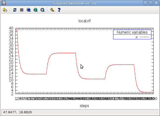
Question: modify the previous program so that x reaches the target after a damped oscillation
like in the following screen-shot:
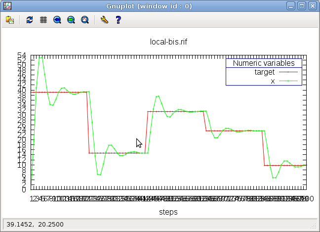
3.13 Damped oscillation
node local() returns(target, x:real = 0.0) =
  exist px : real = 0.0 in -- Because pre pre x is currently not supported in Lutin.
  assert px = pre x in
  loop {
    0.0 < target and target < 42.0 and x = pre x
    fby
    loop [20] {
       x = (pre x + target) / 2.0
           + 0.6*(px - pre px) -- adding inertia...
       and
       target = pre target
    }
  }
3.14 Distribute a constraint into a scope: assert
Now let's consider a slightly different version of the previous
program where n is an input of the node. Since the current
version of the Lutin interpreter is not able to set the previous
value of a variable with an input value (this restriction might
change in the future), we need to write for the first instant a
constraint that does not involve pre cpt.
Consider for instance the true-since-n-instants2.lut program:
node ok_since_n_instants(b:bool;n:int)returns(res:bool)=
  exist cpt: int in
  cpt = n and res = (b and (cpt <= 0))
  fby
     loop {
       cpt = (if b then (pre cpt-1) else n) and
       res = (b and (cpt <= 0))
     }
- One flaw is that
res = (b and (cpt<=0))is duplicated.This occurs very often, for example when you want to a variable to keep its previous value during several steps, and need to write boring
X = pre Xconstraint all the time. Indeed in Lutin, if one says nothing about a variable, it is chosen randomly. - The
assert/inconstruct has been introduced in Lutin to avoid such code duplication.
assert <ce> in <te>≡<te'>,where <te'>= <te>[c/c and ce]\(_{\forall c \in \mathcal{C}onstraints(te)}\)
i.e., where the trace expression <te'> is obtained from the trace
expression <te> by substituting all the constraint expressions
<c> appearing in <te> by the constraint expression <c> and <ce>.
Question: Rewrite the true-since-n-instants2.lut using the
assert/inconstruct and avoid code duplication.
3.15 External code
Lutin program can call any function defined in a shared library (.so)
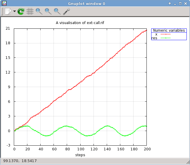
extern sin(x: real) : real
let between(x, min, max : real) : bool = ((min < x) and (x < max))
node bizzare() returns (x,res: real) =
  exist noise: real in
  assert between(noise,-0.1, 0.1) in
  res = 0.0 and x = 0.0 fby
  loop     x = pre x + 0.1 + noise
       and res = sin(pre x)
<prompt> lutin -L libm.so -l 200 ext-call.lut -o ext-call.rif;gnuplot-rif ext-call.rif
3.16 Exceptions
- Global exceptions can be declared outside the main node:
exception ident
- or locally within a trace statement:
exception ident in st
- An existing exception ident can be raised with the statement:
raise ident
- An exception can be caught with the statement:
catch ident in st1 do st2
If the exception is raised in st1, the control immediatelly passes to st2. If the "do" part is omitted, the statement terminates normally.
3.17 Exceptions (cont)
- The predefined Deadlock exception can only be catched
catch Deadlock in st1 do st2
≡
try st1 do st2
- When a trace expression deadlocks, the Deadlock exception is raised. In fact, this exception is internal and cannot be redefined nor raised by the user. The only possible use of the Deadlock in programs is one try to catch it:
- If a deadlock is raised during the execution of st1, the control passes immediately to st2. If st1 terminates normally, the whole statement terminates and the control passes to the sequel.
3.18 Exceptions (cont)
node toto(i:int) returns (x:int)=
  loop {
    exception Stop in
    catch Stop in
       loop [1,10] x = i fby raise Stop fby x = 43
    do x=42
   }
<prompt> luciole-rif lutin except.lut
Note that the 43 value is generated iff i=43.
3.19 Combinators (again)
- Trace Combinators
let myloop(t:trace) : trace = loop try loop t
Here we restart the loop from the beginning whenever we are blocked somewhere inside
t. (myloop.lut)let myloop(t:trace) : trace = loop try loop t node use_myloop(reset:bool) returns(x:int) = myloop( x = 0 fby assert not reset in x = 1 fby x = 2 fby x = 3 fby x = 4 )
<prompt> luciole-rif lutin myloop.lut
Each step you set reset to
true, the output equals to0.
3.20 Parallelism: &>
node n(i:int) returns(x,y:int) = {
      loop { -i < x and x < i }
   &> y = 0 fby loop { y = pre x } }
<prompt> luciole-rif lutin paralel.lut
<te1> &> <te2> executes the trace expression <te1> and <te2> in
parallel.
&>st1 &>... &>stn where the first &> can be omitted. This
statement executes in parallel all the statements st1, …,
stn. All along the parallel execution each branch produces its own
constraint; the conjunction of these local constraints gives the
global constraint. If one branch terminates normally, the other
branches continue. The whole statement terminates when all branches
have terminated.
nota bene: this construct can be expensive because of:
- the control structure: such a product is equivalent to an automata product, which, in the worst case, can be quadratic;
- the data: the polyhedron resolution is exponential in the dimension of the polyhedron.
Use the run/in construct instead if performance is a problem.
4 The run operator
4.1 Cheap parallelism: Calling Lutin nodes run/in
The idea is the following: when one writes:
run (x,y) := foo(a,b) in
in order to be accepted the following rules must hold:
aandbbe uncontrollable variables (e.g., inputs or memories)xandyshould be controllable variables (e.g., outputs or locals)- in the scope of such a
run/in,xandybecomes uncontrollable.
nb : it is exactly the parallelism of Lustre, with an heavier syntax. In Lustre, one would simply write
(x,y)=foo(a,b);
Moreover in Lutin, the order of equations matters.
4.2 Cheap parallelism: Calling Lutin nodes run/in
- The
run/inconstruct is another (cheaper) way of executing code in parallel - The only way of calling Lutin nodes.
- Less powerful: constraints are not merged, but solved in sequence
include "N.lut"
include "incr.lut"
node use_run() returns(x:int) =
  exist a,b : int in
  run a := N() in
  run b := incr(a) in
  run x := incr(b) in
    loop true
<prompt> lutin -l 5 -q run.lut -m use\_run
2
3
4
5
6
The program run.lut illustrates the use of the run/in statements:
This program uses nodes defined in N.lut and incr.lut.
Another illustration of the use of run can be found in the Wearing sensors exemple.
4.3 Why does the run/in statement is important?
Using combinators and &>, it was already possible to reuse code, but
run/in is
- Much more efficient: polyhedra dimension is smaller
- Mode-free (args can be in or out) combinators are error-prone
5 Advanced examples
5.1 Wearing sensors
The sensors.lut program that makes extensive use fo the run statements.
-- Simulate sensors that wears out
node temp_simu_alt (T:real) returns (Ts:real) =
  exist eps : real [-0.1;0.1] in
      Ts = T + eps
   fby
      loop {
          |10: Ts = T + eps     -- working
          |1:  loop Ts = pre Ts -- not working
        }

node temp_simu(T:real) returns (Ts:real) =
  exist eps : real [-0.1;0.1] in
       Ts = T + eps
   fby loop [30,50] Ts = T + eps -- working
   fby loop         Ts = pre Ts  -- not working

node main(Heat_on : bool) returns (T, T1, T2, T3 : real; T1v,T2v,T3v:bool) =
  let delta = 0.2 in
  exist T1_cst, T2_cst, T3_cst : bool = false in
  loop {
    -- init
        T= 7.0 and T1 = T and T2 = T and T3 = T and
        T1v and T2v and T3v
    fby
      let newT = pre T + (if Heat_on then delta else -delta) in
      assert T = newT in
      assert (T1v = (T1 = pre T1)) in
      assert (T2v = (T2 = pre T2)) in
      assert (T3v = (T3 = pre T3)) in

      run T1 := temp_simu(newT) in
      run T2 := temp_simu(newT) in
      run T3 := temp_simu(newT) in
          loop { not (T1 = pre T1 and T2 = pre T2 and T3 = pre T3) }
         -- force to start again from the beginning when the 3 sensors are broken
    }
<prompt> luciole-rif lutin sensors.lut -m main
<prompt> luciole-rif lutin sensors.lut -m main
5.2 Waiting for the stability of a signal
- One of the target application of Lutin is the programming of test scenario of control-command system. In this context, it is often very useful to wait for the stability of a variable (typically, coming from a sensor) before changing again the value associated to a command.
- Defining and checking the stability of a variable (in particular in presence of noise) is not that easy.
- One definition could be that a variable is stable if it remains within an interval during a certain amount of time. More precisely:
A variable V is (d,ε)-stable at instant i if there exists an interval I of size ε, such that, for all n in [i-d,i], V(n) is in I.
∃ I, st |I| = ε, ∀ n ∈ [i-d, i] V(n) ∈ I
- In order to implement such a definition, we'd need to manage n variables; and in order to get parametric code, we'd need arrays. In any case, this is quite expensive (O(n)). Here we propose a lighter version of this test, that is based on the following idea: we test for the stability of the variable during a small amount of instants and hence obtain an interval I; then, we simply check that the variable remains in I for the n-m+1 remaining instants. This is less expensive (O(m) versus O(n)), but of course it is not optimal in the sense that in some cases, we might detect stability a little bit later.
- We now propose a Lutin and a Lustre implementation of this idea.
The Lutin program is fully deterministic, but interestingly enough,
one might find it easier (or not…) to read than the Lustre
equivalent program. This is because Lustre is a purely dataflow
programming language, while Lutin do have explicit control flow
operators (
fby,loop). In the Lustre version ofcompute_ref, we need to encode a 2-states automaton. Such an encoding makes the temporal behavior of the program less explicit.
- The Lutin version
We now paraphrase the isstable.lut Lutin version of this algorithm.
First we define a few constants:
let min(x, y : real) : real = if x < y then x else y
let max(x, y : real) : real = if x > y then x else y
and a few macros:
-- Always loop, even if t deadlocks
let myloop(t:trace) : trace = loop try loop t

-- We flag it as valid after delay consecutive cycles without reset.
Then we define the node
compute_refthat search for (epsilon,small_delay)-stability. This node returns a value of referencevrefthat is equal to the middle of I of a suitable. It also returns a booleanvalidthat becomes true as soon as v is (epsilon,small_delay)-stable, and that remains true as long as v remains in I. Note that I is re-initialiazed as soon as it becomes bigger thatepsilon.node is_d_epsilon_stable(d:int; epsilon, v: real) returns (res:bool) = exist vmin, vmax, diff : real in let init() = (vmin = v) and (vmax = v) and (diff = 0.0) and not res in let step() = vmin = min(v, pre vmin) and vmax = max(v, pre vmax) and diff = ((vmax - vmin) / 2.0) in myloop ( init() fby assert step() and diff <= epsilon in loop [d] not res fby loop res ) node is_d_m_epsilon_stable(d, m:int ; epsilon, v:real) returns (res:bool) = exist stable : bool in run stable := is_d_epsilon_stable(d, epsilon, v) in myloop ( loop { not stable and not res } fby loop [m] { stable and not res } fby
The node
is_stablerests on thecompute_refnode. Whenvalidbecomes true, it waitsbig_delayinstants, and returns true as long asvalidremains true.) node is_stable(v:real) returns (res:bool) = run res := is_d_m_epsilon_stable(3, 5, 3.0, v) -- ca sert à rien le is_d_m_epsilon_stable comparé au is_d_epsilon_stable -- il suffit de prendre d+m et ca fait la meme chose... -- -- un truc plus interessant, serait de coder un is_3_epsilon_stable exacte, -- et de l'utiliser dans is_stable -- exact, and expensive (but for m=3 its ok) node is_3_stable(epsilon, v:real) returns (vref:real;res:bool) = exist v1,v2,v3 : real in v1 = v and v2 = v and v3 = v and not res and vref = v fby assert v1 = v and v2 = pre v1 and v3 = pre v2 and vref = (v1+v2+v3)/3.0 in loop [2] not res fby loop { res = abs(v1-v2)<epsilon and abs(v1-v3)<epsilon and abs(v2-v3)<epsilon } -- this one is an abstraction node is_m_stable(d, m:int ; epsilon, v:real) returns (res:bool) = exist v_average : real in exist vref : real in exist is_stable : bool in run v_average, is_stable := is_3_stable(epsilon,v) in myloop ( loop not is_stable and not res and vref = v_average fby -- on se souvient de la valeur de ref à l'entree de ce loop pour -- détecter une lente dérive de v. assert is_stable and -- as soon it is false, we start from the beginning vref = pre vref and abs(v-vref) < epsilon -- will detect drift in loop [m] not res fby loop res )
<prompt> luciole-rif lutin is\_stable.lut -m is\_stable