Overview
1. Overview
2. Getting started with d/dt
3. References
4. Authors
5. DownloadInput Language
d/dt is a tool for reachability analysis of continuous and hybrid systems with linear differential inclusions.
The tool accepts as input a hybrid automaton where
The problems d/dt can solveContinuous dynamics are linear possibly with uncertain, bounded inputof the form dx/dt = Ax + u where u is input taking values in a bounded convex polyhedron U. All staying conditions ("invariants") and transition guards are defined by convex polyhedra.
All the algorithms implemented in d/dt are presented in [1-0].Representation of Sets: Reachable sets are represented by orthogonal polyhedra [4]. Reachability Technique: The approximation of reachable states is based on numerical integration and polyhedral approximation. The Maximum Principle from optimal control is used to deal with uncertain input in continuous dynamics. See [1, 2, 5, 1-0] for more details on the reachability techniques. Safety Verification Algorithm: Using forward reachability analysis, the tool computes an over-approximationof the reachable set and checks whether it intersects with the bad set. The output is a yes/no answer accompanied by a set of bad states that the system has reached, in case the answer is yes. Switching Controller Synthesis Algorithm: The tool computes an under-approximation of the maximal invariant set (see 2, 1-0]) and derives from this set the switching control laws that restrict the staying conditions and transition guards of the original hybrid automaton so that the resulting automaton meets the desired safety specification.
2. Getting started with d/dt
The input system and its specifications are defined in a file with .hyb extension, called the model file. The syntax of the description language is described here. You can also specify some computation parameters in a file with .par extension. The tuning of the computation parameters can help to achieve better compromise between accuracy and performance. If the parameter file does not exist for a given model file, default parameters are used (but the quality of approximation can be bad).Before starting the analysis you need to:
1. Define the system and its safety specification (a bad set or a safe set) in a file with .hyb extension, e.g. example1.hyb.2. Specify the computation parameters in example1.par.
ddt [options] [modelname]modelname is the name of the model file (with .hyb extension, e.g. example1.hyb) which contains the description of the input hybrid automaton. As mentioned above, computation parameters will be read from the file example1.par.
The following options are available. Note that
the options in the command line override those defined in the parameter
files.
PbType = reach: the tool computes an over-approximation of the set of all states reachable from the initial set.
PbType = verif: the tool checks whether the system satifies the safety property specified as a set of bad states. If no such sets are specified, only the computation of the reachable set is performed.
RepType = uni: orthogonal polyhedra are encoded by matrices (implemented using dictionary arrays), and the underlying grid is uniform with fixed size.
RepType = grid: orthogonal polyhedra are encoded by their extreme vertices, and the size of the underlying grid is variable.
If unspecified the option grid will be used.
Tip: In general, the griddy implementation is more stable. However, for low dimensional systems, the uniform implementation is more time efficient.
ViewMode = noview: no run-time visualization of the results.
ViewMode = geomview: evoke GeomView (which is a free professional 3D viewer) to display the results that d/dt sends to GeomView via pipe communication. To use this option, GeomView must be priorily installed.
ViewMode = ddt_viewer: use the viewer of d/dt. This viewer is simple and does not include advanced 3D features (in order to save computation time). For a better visualization quality, use geomview option.
If unspecified, the viewer of d/dt will be used.
Example
When executing ``ddt
-v geomview -o data/example1.hyb'', d/dt
performs reachability analysis on the system described in file example1.hyb
in directory data.
In case of syntax errors,
d/dt
refuses
and writes out a message. GeomView is evoked to visualize
the reachable set, and once the computation terminates the results are
saved in data/example1.res.
As another example, when executing ``ddt
-p verif -v noview data/example1.hyb'', in
addition to the reachability computation, the tool checks whether the system
satisfies the safety property. No run-time visualization is used, and the
results will not be saved.
Running d/dt with the menu bar
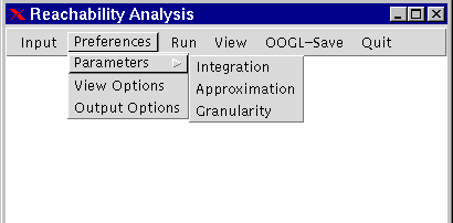
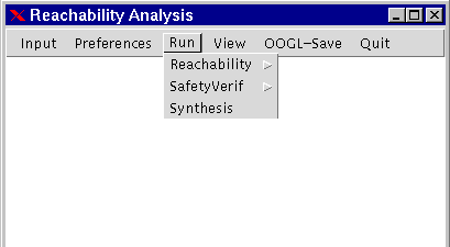
A more interactive way of using d/dt is to evoke its menu bar by executing the command ``ddt'' (without options and modelname). The menu bar consists of 5 submenus:
Input: used to select the model file.
Run: used to select the type of analysis and start the analysis.
Preferences: During the analysis of a system, some computation parameters and options can be modified via the {\tt Preferences} menu without changing the parameter file.
View: this menu allows to display the results from the output files .res. This is useful when the user might wish to skip run-time visualization in order to reduce computation time. The reachable set at each location will be displayed. Press the right button of the mouse in the display windowto change the location to display or to go back to the main menu. Press, hold and move the left/middle mouse button in the display window (or use the key-left/right/down/up) to rotate the displayed object.
OOGL-Save: this menu is used to transform results stored in output files .res into OOGL (Object Oriented Graphics Language) format data, which can be then input to GeomView.
To use the tool with the menu bar,


A snapshot of the graphical interface
3. References
4. Authors Thao Dang and Oded Maler
Acknowledgements: Eugene
Asarin had a great contribution to the ideas of d/dt. We used the library
Cubes of Olivier Bournez. The
treatment of continuous dynamics with disturbances was inspired by the
work [3] of Pravin
Varaiya.
We also used the library LEDA,
the convex polyhedral packages cdd
and Qhull,
the linear programming solver lp_solve,
the ODE solver CVode,
and the 3D graphics library Mesa.
This work was supported by the European project
VHS
(ESPRIT-LTR 26270).
5. Download
If you're interested in using d/dt, please
send us an email (thao.dang@imag.fr).
.